


Want to get more out of Excel? At Microsoft's inauguralData Insights Summitlast month, several experts offered a slew of suggestions for getting the most out of Excel 2016. Here are 10 of the best.
(Note: Keyboard shortcuts will work for the 2016 versions of Excel, including Mac; those were the versions tested. And many of the query options in Excel 2016's data tab come from the Power Query add-in for Excel 2010 and 2013. So if you've got Power Query on an earlier version of Excel on Windows, a lot of these tips will work for you as well, although they may not work on Excel for Mac.)
1. Use a shortcut to create a table.表是在Excel中最有用的功能数据是在连续的列和行中。表更容易排序,过滤器和可视化,以及添加保持相同的格式上面摆着行新行。此外,如果您从数据生成图表,使用表意味着,如果你添加新行的图表将自动更新。
+RELATED:15 simple, yet powerful Excel functions you need to know+
If you've been creating tables from your data by going to the Excel ribbon, clicking Insert and then Table, there's an easy keyboard shortcut: After first selecting all your data with Ctrl-A (command-shift-spacebar for Mac), turn it into a table with Ctrl-T (command-T on Mac).
Bonus tip: Make sure to rename your table to something related to your specific data, instead of leaving the default titles Table1 or Table2. Your future self will thank you if you need to access that information from a new, more complex workbook.
2. Add a summary row to a table.您可以通过检查新增摘要列在Windows上的设计色带或色带表在Mac上一表“汇总行。”计数,标准偏差,平均多:虽然它叫总计行,你可以从各种汇总统计的,不只是一个总和选择。
虽然你当然可以用一个公式手动插入此信息到电子表格,把信息的汇总行意味着它的“附加”到你的餐桌,但会停留在底部行中,无论你怎么那么可能会选择将表中的数据进行排序。如果你正在做大量的数据探索这可能是很方便。
Note that you'll need to create a total row for each column individually; creating a sum for one column won't automatically generate sums for the rest of your table (since not all columns may have the same type of data -- a sum for a column of dates wouldn't make much sense, for example).
3. Easily select columns and rows.If your data is in a table and you need to refer to an entire column in a new formula, click on the column name. That will give a reference to the full column by name -- useful if you later add more rows to the table, because you won't have to readjust a more specific reference such as B2:B194.
Note: It's important to make sure your cursor looks like a down arrow before you click on the column name. If your cursor looks like a cross when you do so, you'll get a reference to just that lone cell, not to the whole column.
无论您的数据是在一个表中,有一对夫妇选择方便快捷,你可以使用:Shift +空格键选择整行和Ctrl +空格键(或控制+空格键在Mac)来选择整列。请注意,如果你的数据不是在一个表中,这些选择超越现有的数据和包括任何空单元格超越。对于表数据时,选择停在表格的边框。
If you want to select an entire column that's not in a table with just the cells that have data in them, put your cursor in a column next to it, hit Ctrl-down arrow, use the right or left arrow key to move to your desired column, and then hit Ctrl-Shift-up (use command instead of Ctrl on a Mac). This can be handy if your data column is quite long.
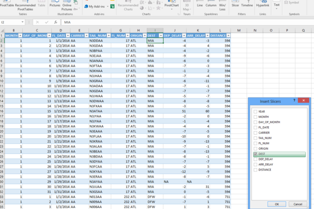
4. Filter table data with slicers.Excel表格提供下拉箭头旁边的每个列标题为容易的排序,搜索和过滤。但是,试图与小的下拉过滤器数据,当你有大量的项目可以是有点麻烦。一些在数据洞察首脑会议主持人建议使用切片机来代替。
"Anybody who sends you a pivot table without slicers, you should teach them slicers in 30 seconds. People love slicers," said Indiana University professor Wayne Winston, who also advises Dallas Mavericks owner Mark Cuban on basketball stats.
虽然切片机最初是为πvot tables, they now work on "regular" tables as well (and have since Excel 2013 on Windows). "This is actually more useful," Winston argued. (Slicers are available for pivot tables but not regular tables in Excel for Mac 2016.)
To add a slicer to a table, with your cursor already somewhere in the table, head to the Design ribbon, select Insert Slicer and then choose which column(s) you'd like to filter.
限幅器将显示在您的工作表中,出现一列宽只有少数项目展示。但是,如果你有很多的空间你的数据右侧的狭长的电子表格,你可以调整切片器比默认的宽得多。您可以在功能区中的切片器选项中列添加到切片机布局。
如果你想在一个切片多个项目过滤器,按住Ctrl键单击。要清除所有过滤器,还有在切片机的右上角清晰的按钮。
5.创建更改时您筛选表的汇总细胞。如果创建一个表中总结了数据的表外的单元格 - 一列的总和,例如 - 你会喜欢的小区,如果你的东西过滤表中显示更新的总和,一个基本公式SUM将无法正常工作。
Instead of simply using SUM in that cell, use the你的细胞内骨料功能, and then your cell can be linked to your table filters.

Excel的骨料功能需要三个参数,其中两个是数字。Excel的Windows提供了可用选项的列表。
AGGREGATE requires three arguments: A function number, a desired option number and the range of cells you want to operate on. Type=AGGREGATE(in Excel for Windows and you'll see the available functions and options; in Excel for Mac, you'll have to click on the AGGREGATE help function in order to see available function and option numbers.
SUM is function number 9; ignore hidden rows is option 5. So, a cell with the following code:
=AGGREGATE(9,5,Table1[Expenditures])
gives you the sum of allvisiblerows only. If a filter changes which rows are visible, your sum will change accordingly.

骨料报价仅总结可见行的选项。
6.一种在枢轴表排序的数据。Sometimes you'd like to sort data by a specific column in a pivot table -- just as with a regular table. But unlike regular tables, pivot tables don't have dropdown menus on each column offering the ability to sort. However, if you choose the lone dropdown arrow on the first column, you'll get a menu allowing you to sort by any column.
7.“逆透视”的数据。Some call thisreshaping data from "wide" to "long"。In the database world, it's known as "fold": Taking data from individual columns and moving them into rows. Basically, it's the opposite of creating a pivot table -- in a pivot table, you pull categories within one column up into their own columns.
To unpivot columns, you need to use the Query Editor in Excel 2016. Access the Query Editor via the Data ribbon: In the Get & Transform section, choose From Table.
Once the Query Editor comes up (if your data isn't already in a table, you'll be asked to confirm a data range first), select the columns you want to unpivot, click on the Transform tab and chose Unpivot Columns.
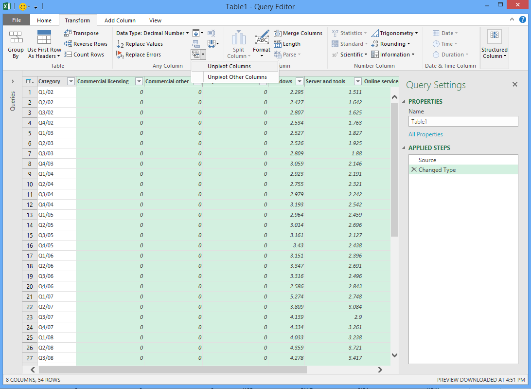
Excel的查询编辑器为用户提供了选项逆透视列。
That will create two new columns at the right of your spreadsheet, Attribute and Value, with the columns you unpivoted. You can rename those columns to something that makes more sense, such as "Product" and "Price" or "Quarter" and "Revenue."
To save your work, selectFile > Close & Load(to the default destination) or文件>关闭并载入至in order to be asked where you'd like to save your results. If you try to close without saving, you'll be asked whether you want to keep your changes; say Yes and they'll be saved on a new worksheet.

Unpivoting data turns a wide table into a longer one, combining multiple columns into two: attribute (category) and value.
Microsoft Office网站有在unpivoting更多信息。
8. Make multiple pivot tables for one column of categories.If you have a pivot table and add a filter for one column that contains categories, you can generate copies of that pivot table, one for each category in your filter, by going toAnalyze > Options > Show Report Filter Pagesand then selecting the filter you want. This can be handier than having to click through each category in your filter manually.
(在Excel的2016年Mac,请到数据透视表功能区上的分析标签,然后选择Options > Show Report Filter Pages。)
9. Look up data with INDEX MATCH.While VLOOKUP is a popular way to find data in one Excel table and insert it into another, INDEX combined with MATCH can be more powerful and flexible. Here's how to use them.
比方说,你在那里有一个列有计算机模型名称的查找表,列B有价格信息,和列d也是在那里你要添加价格信息的计算机模型的名称。创建使用此格式的公式:
= INDEX(ColumnToSearchForValue,MATCH(CellWithLookupKey,ColumnToSearchForLookupKey,0)
样品可能是这样的:
= INDEX(B2:B73,MATCH(D2,A2:A73,0))
This is how/why INDEX MATCH works (if you don't need to know, skip to the next tip): INDEX selects a specific cell by numerical location. You first give it a range of cells, either within a single column or a single row, and then tell it the specific number of the cell you want.
例如,你可以挑选第6项B列有:
=INDEX(B2:B19, 6)。
你会使用以下格式:
=INDEX(ColumnOrRowToSearch, ItemNumberInThatColumnOrRow)
However, using INDEX alone isn't much help if you want to find a value based on some condition in another column. That is, you don't want the 6th item in your Price column B; you want the item in your Price column that matches something in column A, such as a certain computer model.
That's where MATCH comes in. MATCH searches for a value in a range of cells and returns the location of what's matched, using the following format:
=MATCH(SearchValue,RangeToSearch,MatchType)
(匹配类型可以是0,完全相等,1最大值小于或等于你正在搜寻或-1,大于或等于您查找值的最小值)。
所以,如果你想找到在B列的单元格正是999的位置,你可以使用:
=MATCH(999, B2:B79, 0)。
And, so the combination: MATCH, looking for a specific value based on a search term, returns a cell location; and INDEX needs a location as its second formula argument.
10.观看一个公式(仅对Windows)来评价步步。Have a complicated formula? If you want to see how it gets evaluated, go toFormulas > Evaluate Formulato see the calculations run step by step.
11. Import and refresh data from the Web into Excel.这个工作最好,当你有一个Web页面上的格式良好的HTML表格;更多的自由格式的文本(甚至是格式不表),你需要做额外的编辑相当数量,让您的数据转换成可以分析的形式。
随着该警告记住,如果你想从Web到Excel,头在Excel中的数据标签用于Windows和选择拉一个HTML表格:New Query > From Other Sources > From Web
Enter the URL of the appropriate Web page. Excel will look for and list available HTML tables on that page. Click on a table to see a preview; when you find the one you want, click Load.
为什么不珍ust copy and paste a well-formatted HTML table into Excel? If the data updates frequently, you can easily refresh it by right-clicking in the table and selecting Refresh instead of having to copy and paste new data.
For more on the conference, check out theYouTube上的Microsoft数据洞察视频。
这个故事,“11个的Excel技巧超级用户”最初发表计算机世界 。